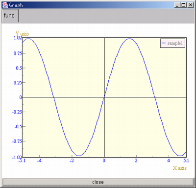
図 2.2 表示されたグラフ
このライブラリの目玉である可視化・グラフ関係と数値計算関係について、簡単なコーディング例を用いて説明します。それぞれの詳しい説明は部[各機能解説]やAPIドキュメントを参照してください。
関数についての詳しい説明は後述の節[関数を作る]を参照してください。(3)
まず、三角関数sinのグラフを表示します。
import ccs.math.*;
import ccs.comp.ngraph.*;

class HowtoFunc1 {
	public static void main(String [] args) {
		//関数を作って
		AFunction f = AFunctionClass.getFunction("sin(x)");
		//表示
		Graph.show(f);
	}
}
実際、本質的な部分は2行です。
以下のようにコンパイルして、実行します。
% javac HowtoFunc1.java
% java HowtoFunc1
この結果は以下のようです。
いろいろ細かく調整する場合は、グラフのオブジェクト(PlotContext)を取得する必要があります。方法は以下のようにGraphクラスを使う方法と、自分で構築する方法の2種類あります。
PlotContext context = Graph.show( f );
この方法は手軽で簡単です。
import java.awt.*;
import ccs.math.*;
import ccs.comp.ngraph.*;
import ccs.comp.ngraph.d2.*;

class HowtoFunc2 {
	public static void main(String [] args) {
		//関数を作って
		AFunction f = AFunctionClass.getFunction("sin(x)");

		//構築
		PlotContext2D context = new PlotContext2D();
		PlotData d = new FunctionData2D( f );
		d.setDataName("function : sin(x)");
		context.addPlotter( new LinePlotter( d ) );

		//AWTコンポーネント作成
		PlotRenderer renderer = new SquarePlotRenderer2D(context);
		AWTPlotComponent pc = new AWTPlotComponent(600,500);
		pc.addRenderer(renderer);

		//画面に表示
		Frame t = new Frame("graph test");
		t.add("Center", pc );
		t.pack();
		t.show();
	}
}
この方法は多くのクラスを扱うことになりますが、微妙な調整がやりやすいです。これらのクラスの詳しい使い方は、以降のHowtoや、各機能解説を参照してください。
ファイルからデータを読み込み、データから関数(AFunction)に変換してしまって、前述の方法でグラフに出すのが簡単です。
$ cat data1.dat
0 1
1 3
2 6
3 10
4 4
5 0
6 1
import ccs.math.*;
import ccs.math.util.*;
import ccs.comp.ngraph.*;

class HowtoFile2Graph1 {

	public static void main(String [] args) {
		//データ読み込み
		DataArraySet ds = Loader.load("data1.dat");
		//関数に変換
		AFunction f = new AArrayFunction(ds.getColumn(0),ds.getColumn(1));
		//表示
		Graph.show(f);
	}
}
Loaderは、数値データの並んだファイルを配列のオブジェクト(DataArraySet)にするユーティリティーです(参照:###)。AArrayFunctionは、配列を関数に見せかけるラッパークラスです。配列の範囲外の扱いや補完などを設定できます(参照:###)。
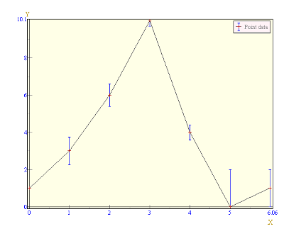
この方法は関数として表示してしまうので線でしか表示できません。データ点を点や記号で表示するには以下のように自分でオブジェクトを構築して細かく指定します。
import java.awt.*;
import ccs.math.*;
import ccs.math.util.*;
import ccs.comp.ngraph.*;
import ccs.comp.ngraph.d2.*;

class HowtoFile2Graph2 {
	public static void main(String [] args) {
		//データ読み込み
		DataArraySet ds = Loader.load("data1.dat");

		//構築
		PlotContext2D context = new PlotContext2D();
		PlotData d = new XYData2D( ds.getColumn(0),ds.getColumn(1) );
		d.setDataName("Point data");
		context.addPlotter( new IconPlotter( new LinePlotter( d ) ) );

		//AWTコンポーネント作成
		PlotRenderer renderer = new SquarePlotRenderer2D(context);
		AWTPlotComponent pc = new AWTPlotComponent(600,500);
		pc.addRenderer(renderer);

		//画面に表示
		Frame t = new Frame("graph test");
		t.add("Center", pc );
		t.pack();
		t.show();
	}
}
Plotterのサブクラスでプロット方法を指定します。クラスを多段に構築することで、プロット方法を組み合わせることが出来ます。(参照:###)
エラーバーが必要であれば、以下のようにエラーバー用のクラスを使います。
import java.awt.*;
import ccs.math.*;
import ccs.math.util.*;
import ccs.comp.ngraph.*;
import ccs.comp.ngraph.d2.*;

class HowtoFile2Graph3 {
	public static void main(String [] args) {
		//データ読み込み
		DataArraySet ds = Loader.load("data2.dat");

		//構築
		PlotContext2D context = new PlotContext2D();
		PlotData d = new XYErrorData2D(ds.getColumn(0),ds.getColumn(1),
									   ds.getColumn(2));//誤差付データ構築
		d.setDataName("Point data");
		context.addPlotter
			( new IconPlotter( new LinePlotter
				( new ErrorBarPlotter(d) ) ) );//誤差幅描画クラス

		//AWTコンポーネント作成
		PlotRenderer renderer = new SquarePlotRenderer2D(context);
		AWTPlotComponent pc = new AWTPlotComponent(600,500);
		pc.addRenderer(renderer);

		//画面に表示
		Frame t = new Frame("graph test");
		t.add("Center", pc );
		t.pack();
		t.show();
	}
}
$ cat data2.dat
0 1  1
1 3  1.5
2 6  1.2
3 10 0.6
4 4  0.8
5 0  4
6 1  2
このあと、続けて曲線での補完やフィッティングも可能です。(参照:###)
まず、PlotContextのオブジェクトを取得します。取得の方法は、自分で構築するか、Graphクラスのshowメソッドの帰り値がPlotContextのオブジェクトですのでこれを使います。
次に、以下のようにPlotContextの自動範囲調整を解除させて表示範囲を設定し、更新メソッドを呼びます。
//PlotContext context
context.setAutoScale(0,false);//x軸の自動調整を解除
context.setAutoScale(1,false);//y軸の自動調整を解除
context.setActiveRange(new RealRange(-3,-4,6,8));
// RealRangeの引数 => 左側x座標、下側y座標、x方向の幅、y方向の幅

context.updatePlotter();//表示更新
setAutoScaleで解除しなかった軸には、setActiveRangeで範囲を指定しても無視されます。
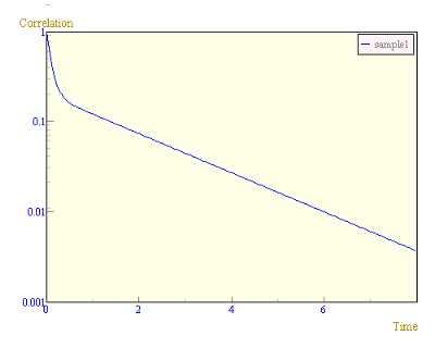
Logスケールや軸目盛りについては節[軸関係]を参照してください。
軸に関して設定できる項目は、Logスケール、軸ラベル、軸目盛りです。
PlotContextのgetAxis(dimension)から、設定したい軸のAxisオブジェクトを取得して操作します。
Logスケールは、setLogメソッドで行いますが、Logスケールにした時に表示範囲やデータがLogで表示できる範囲である必要があります。
軸ラベルはsetLabelで行います。
軸目盛りはGridGeneratorインターフェイスを実装したオブジェクトが指定します。(参照:###)
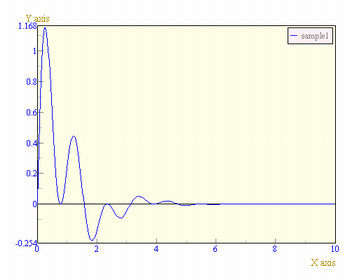
import ccs.math.*;
import ccs.comp.ngraph.*;

class HowtoAxisGrid {

	public static void main(String [] args) {
		AFunction f =
			AFunctionClass.getFunction("0.8*exp(-10*x)+0.2*exp(-0.5*x)");
		//PlotContext 取得
		PlotContext context = Graph.show(f);
		context.setAutoScale(0,false);
		context.setAutoScale(1,false);
		context.setActiveRange( new RealRange(0,0.001,8,1) );
		//Axis取得
		Axis xAxis = context.getAxis(0);
		Axis yAxis = context.getAxis(1);
		//X軸の設定
		xAxis.setLabel("Time");
		//    主目盛り 0から2刻み
		xAxis.setMainGridGenerator(new CustomGridGenerator(0,2));
		//    副目盛り 0から1刻み
		xAxis.setSubGridGenerator(new CustomGridGenerator(0,1));
		//Y軸の設定
		yAxis.setLabel("Correlation");
		//    Logスケール
		yAxis.setLog(true);
		//更新
		context.updatePlotter();
		System.out.println(context.getActiveRange());
	}

}
グラフの見た目に関わるパラメーターは、SquarePlotRenderingParamで行います。ここで設定できる主な項目は、余白、凡例の位置、グリッド線、背景の描画方法、フォント、各種色です。
import java.awt.*;
import ccs.math.*;
import ccs.comp.*;
import ccs.comp.ngraph.*;
import ccs.comp.ngraph.d2.*;

class HowtoGraphParam {

	public static void main(String [] args) {
		//関数を作って
		String function = "exp(-0.5*x)*sin(x)+random(2)";
		AFunction f = AFunctionClass.getFunction(function);
		//構築
		PlotContext2D context = new PlotContext2D();
		PlotData d = new FunctionData2D( f );
		d.setDataName(function);
		context.addPlotter( new LinePlotter( d ) );
		//AWTコンポーネント作成
		SquarePlotRenderer2D renderer = new SquarePlotRenderer2D(context);
		AWTPlotComponent pc = new AWTPlotComponent(600,500);
		pc.addRenderer(renderer);

		//見た目の設定
		SquarePlotRenderingParam param = renderer.getRenderingParam();
		//   背景の設定
		param.wholeBackgroundPainter = new ImagePainter("sampleImage.jpg",ImagePainter.FIT,pc);
		param.contentBackgroundPainter = new DefaultRectPainter(new Color(255,255,255,180));
		param.legendBackgroundPainter = new DefaultRectPainter(Color.white);
		//   グリッド線を引く
		param.mainXGridWholeLine = true;
		param.mainYGridWholeLine = true;
		//   フォントの設定
		param.legendFont = new Font("SansSerif",Font.PLAIN,14);
		param.labelFont = new Font("SansSerif",Font.BOLD,22);
		param.gridFont = new Font("SansSerif",Font.BOLD,20);
		//   色の設定
		param.axisLabelColor = Color.black;
		param.legendLabelColor = Color.red;
		param.gridLabelColor = Color.black;

		//画面に表示
		Frame t = new WFrame("graph test");
		t.add("Center", pc );
		t.pack();
		t.show();
	}
}

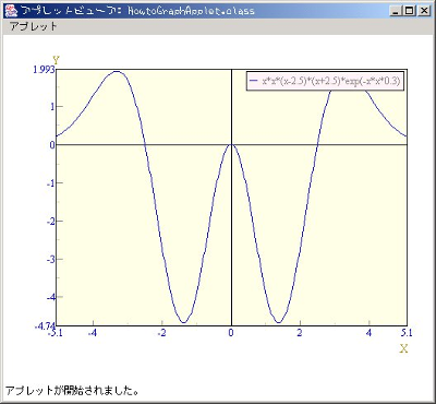
CCSライブラリをアプレットで使うには以下の手順が必要です。
まず、普通にアプレットのソースを書きます。以下簡単な例です。
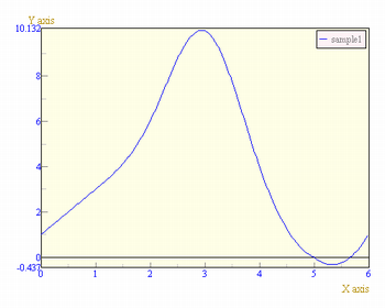
import java.applet.*;
import ccs.math.*;
import ccs.comp.ngraph.*;
import ccs.comp.ngraph.d2.*;

/*
  <applet archive="sample.jar" code="HowtoGraphApplet.class" width="520" height="420">
  </applet>
 */

public class HowtoGraphApplet extends Applet {

	public void init() {
		String function = "x*x*(x-2.5)*(x+2.5)*exp(-x*x*0.3)";
		//関数を作って
		AFunction f = AFunctionClass.getFunction(function);

		//構築
		PlotContext2D context = new PlotContext2D();
		PlotData d = new FunctionData2D( f );
		d.setDataName(function);
		context.addPlotter( new LinePlotter( d ) );

		//AWTコンポーネント作成
		PlotRenderer renderer = new SquarePlotRenderer2D(context);
		AWTPlotComponent pc = new AWTPlotComponent(500,400);
		pc.addRenderer(renderer);

		//コンポーネントの登録
		add(pc);
	}

}
これをコンパイルして、JDK付属のjarというツールでccs.jarと一緒にパッケージにまとめます。
$ ls
HowtoGraphApplet.java    HowtoGraphApplet.class
$ cp (ライブラリがある場所)/ccs.jar sample.jar
$ jar uvf sample.jar HowtoGraphApplet.class
HowtoGraphApplet.class を追加中です。(入 = 1210) (出 = 647)(46% 収縮されました)
あとは、このsample.jarをHTMLファイルのある場所に置きます。HTMLファイルに次のように書けばブラウザの中でアプレットが動きます。
<applet archive="sample.jar" code="HowtoGraphApplet.class" width="520" \
    height="420">
  </applet>
PlotDataのデータを変更して、PlotContext.updatePlotter()を呼ぶと更新されます。適当なタイミングでこれらを呼び出して、グラフを動かします。
import java.awt.*;
import ccs.math.*;
import ccs.comp.ngraph.*;
import ccs.comp.ngraph.d2.*;

class HowtoGraphTime {
	public static void main(String [] args) {
		double [] xx = {1,2,3,4,5};
		double [] yy = {1,2,3,4,5};

		//構築
		PlotContext2D context = new PlotContext2D();
		XYData2D d = new XYData2D( xx,yy );
		d.setDataName("Point data");
		context.addPlotter( new IconPlotter( new LinePlotter( d ) ) );

		//AWTコンポーネント作成
		PlotRenderer renderer = new SquarePlotRenderer2D(context);
		AWTPlotComponent pc = new AWTPlotComponent(600,500);
		pc.addRenderer(renderer);

		//画面に表示
		Frame t = new Frame("graph test");
		t.add("Center", pc );
		t.pack();
		t.show();

		//画面書き換えのスレッド開始
		Thread thread = new Thread(new ValueChanger(xx,yy,d,context));
		thread.start();
	}

	static class ValueChanger implements Runnable {
		private double [] xx;
		private double [] yy;
		private XYData2D data;
		private PlotContext plotContext;
		ValueChanger(double [] xx,double [] yy,XYData2D data,PlotContext pc) {
			this.xx = xx;
			this.yy = yy;
			this.data = data;
			this.plotContext = pc;
		}
		public void run() {
			try {
				//無限ループを起こす
				while(true){
					//データを適当に更新する
					for (int i=0;i<yy.length;i++) {
						yy[i] = Math.random()*5;
					}
					data.setData(xx,yy);
					plotContext.updatePlotter();//画面更新
					Thread.sleep(400);//0.4秒停止
				}
			} catch (Exception e) {
				e.printStackTrace();
			}
		}
	}
}
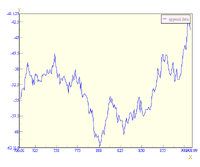
別の要求として、新しい値を追記していくグラフもあります。一定時間ごとに新しい値を観測してグラフに加えていきます。
import java.awt.*;
import ccs.math.*;
import ccs.comp.ngraph.*;
import ccs.comp.ngraph.d2.*;
import java.util.Random;

class HowtoGraphAppend {
	public static void main(String [] args) {
		//構築
		PlotContext2D context = new PlotContext2D();
		AdditiveData2D d = new AdditiveData2D();
		d.setDataName("append data");
		context.addPlotter( new LinePlotter( d ) );

		//AWTコンポーネント作成
		PlotRenderer renderer = new SquarePlotRenderer2D(context);
		AWTPlotComponent pc = new AWTPlotComponent(600,500);
		pc.addRenderer(renderer);

		//画面に表示
		Frame t = new Frame("graph test");
		t.add("Center", pc );
		t.pack();
		t.show();

		//画面書き換えのスレッド開始
		Thread thread = new Thread(new ValueAppender(d,context));
		thread.start();
	}

	static class ValueAppender implements Runnable {
		private AdditiveData2D data;
		private PlotContext plotContext;
		ValueAppender(AdditiveData2D data,PlotContext pc) {
			this.data = data;
			this.plotContext = pc;
		}
		public void run() {
			try {
				Random gen = new Random();
				int count = 0;
				double p = 0;
				//無限ループを起こす
				while(true){
					//データを適当に更新する
					p += gen.nextGaussian();
					data.add(count++, p);
					plotContext.updatePlotter();//画面更新
					Thread.sleep(80);//0.08秒停止
				}
			} catch (Exception e) {
				e.printStackTrace();
			}
		}
	}
}
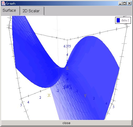
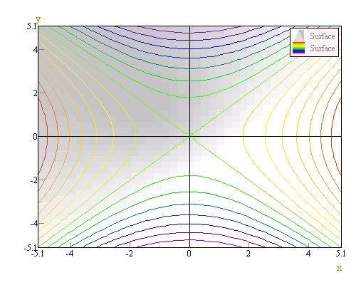
3次元のプロットを以下のような方法で行うことが出来ます。軸や表示範囲などはこれまでの方法が応用できます。ここでは簡単なコード例を示します。
import ccs.comp.ngraph.*;
import ccs.math.*;

public class Howto3DSimple {

	public static void main(String [] arg) {
		String exp = "(x*x-y*y)/4";
		ScalarFunction func = ScalarFunctionClass.getFunction(exp);
		Graph.show(func);
	}
}
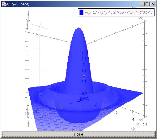
import ccs.comp.ngraph.d3.*;
import ccs.comp.ngraph.*;
import ccs.math.*;
import ccs.comp.WFrame;
import ccs.comp.d3.*;
import java.awt.*;

public class Howto3DSurface {

	public static void main(String [] arg) {
		Frame f = new WFrame("graph test");
		f.add("Center",getComponent());
		f.pack();
		f.show();
	}

	static Component getComponent() {
		PlotContext3D context = new PlotContext3D();
		String form2 = "exp(-(x*x+y*y)*0.2)*cos( (x*x+y*y)*0.5)*3";
		ScalarFunction func2 = ScalarFunctionClass.getFunction(form2);
		SurfaceFunctionData3D data2 = new SurfaceFunctionData3D(func2);
		data2.setDataName(form2);
		data2.setDivision(40);
		Plotter3D plotter2 = new SurfacePainter3D(data2);
		context.addPlotter(plotter2);

		return UGraph.setup3DRenderer(context).getComponent();
	}
}
さらに詳しい内容は、詳細###を参照してください。
グラフを表示させたり、各種演算を行うには関数オブジェクトが必要になります。関数オブジェクトは要するに「ある値を与えると、何かしらの値を出力する機能を有するオブジェクト」です(4)。
関数オブジェクトの構築の仕方には文字列、継承、無名クラスからの3種類あります。
文字列から構築する方法が一番簡単ですが、実行速度が多少犠牲になります。使える関数や演算子については、詳細###を参照してください。
AFunction function = AFunctionClass.getFunction("sin(x)*x");
関数の基底クラスAFunctionを継承するのが普通の使い方です。ただ、単純な機能の関数を構築するのであれば、次の無名クラスのほうが楽です。
//どこか適当なところで定義
class SomeFunction extends AFunction {
    public double f(double x) {
         return Math.sin(x)*x;
    }
}

//必要なところで構築
AFunction function = new SomeFunction();
無名クラスは名前をつけて定義しなくて済むので、コーディング量が少なくて済みます。
//必要なところでいきなり構築
AFunction function = new AFunction() {
    public double f(double x) {
        return Math.sin(x)*x;
    }
};
ちなみに、関数にはスカラー関数とベクトル関数があります。スカラー関数の中に引数を一つだけ取る一次元関数(今回用いたAFunction)が特別に用意してあります。多くの場面ではこの一次元関数を使います。(参照:###)
現在では、1次元のデータの読込みのみサポートしています。以下のようなデータを読み込んで関数を構築します。
$ cat data1.dat
0 1
1 3
2 6
3 10
4 4
5 0
6 1
import ccs.math.*;
import ccs.math.util.*;
import ccs.comp.ngraph.*;

class HowtoFile2Func1 {

	public static void main(String [] args) {
		//データ読み込み
		DataArraySet ds = Loader.load("data1.dat");

		//データ配列へのアクセス
		System.out.println("列数:"+ds.getColumn());
		System.out.println("行数:"+ds.getRow());
		double [][] ar = ds.getArray();
		for(int i=0;i<ar[0].length;i++){
			for (int j=0;j<ar.length;j++ ) {
				System.out.print(ar[j][i]);
				if (j < (ar.length-1)) {
					System.out.print(" : ");
				}
			}
			System.out.println();
		}

		//関数に変換
		AArrayFunction f = new AArrayFunction(ds.getColumn(0),ds.getColumn(1));
		f.setInterpolater( new SplineInterpolater());//spline補完
		AFunction af = AFunctionClass.wrap(f);//普通の関数に見せかける

		//表示
		PlotContext context = Graph.show(af);
		context.setAutoScale(0,false);
		context.setActiveRange( new RealRange(0,0.001,6,1) );
		context.updatePlotter();
	}
}
$ java HowtoFile2Func1
列数:2
行数:7
0.0 : 1.0
1.0 : 3.0
2.0 : 6.0
3.0 : 10.0
4.0 : 4.0
5.0 : 0.0
6.0 : 1.0
微分・積分にはいくつかのアルゴリズムがあります。(参照:###)基本的に演算子を取り替えるだけで別のアルゴリズムを利用可能です。
import ccs.math.*;
import ccs.math.dif.*;

public class HowtoDiff {

	public static void main(String [] args) {
		//関数
		AFunction func = AFunctionClass.getFunction("sin(x)");
		//微分演算オブジェクト : Richardson加速法(差分0.05, 反復1回)
		ADifferentiator dif = new RichardsonIterDifferentiator(0.05,1);
		//微分実行 x=0 で微分
		System.out.println( dif.point( 0 ).operate(func) );

		//精度を上げてみる
		dif = new RichardsonIterDifferentiator(0.05, 2);
		System.out.println( dif.point( 0 ).operate(func) );
	}

}
$ java HowtoDiff
0.9999999869801355
0.9999999999999515
import ccs.math.*;
import ccs.math.integral.*;

public class HowtoInt {

	public static void main(String [] args) {
		//関数
		AFunction func = AFunctionClass.getFunction("sin(x)");
		//積分演算オブジェクト : 台形公式
		AIntegrator it = new TrapezoidalIntegrator(0.05);
		//微分実行 x=0~PI で積分
		System.out.println( it.range( 0, Math.PI ).operate(func) + " : " + it.getClass().getName() );

		//アルゴリズムを取り替えてみる
		it = new SimpsonIntegrator(0.05);
		System.out.println( it.range( 0, Math.PI ).operate(func) + " : " + it.getClass().getName() );
		it = new RichardsonIntegrator(0.05);
		System.out.println( it.range( 0, Math.PI ).operate(func) + " : " + it.getClass().getName() );
		it = new Gauss10Integrator();
		System.out.println( it.range( 0, Math.PI ).operate(func) + " : " + it.getClass().getName() );
		it = new DEIntegrator(0.05);
		System.out.println( it.range( 0, Math.PI ).operate(func) + " : " + it.getClass().getName() );
	}

}
$ java HowtoInt
1.9976791298681702 : ccs.math.integral.TrapezoidalIntegrator
2.0000000732694567 : ccs.math.integral.SimpsonIntegrator
1.998442208667804 : ccs.math.integral.RichardsonIntegrator
2.0 : ccs.math.integral.Gauss10Integrator
1.9999999999999998 : ccs.math.integral.DEIntegrator
また、導関数、積分関数を返すメソッドがありますので、それを用いると便利な時があります。文字列から構築した関数の場合は、代数計算を行って出来るだけ解析的に計算します。簡単に計算出来ない場合や、AFunctionなどを実装した関数の場合は適当な演算子で数値的に計算します。
import ccs.math.*;
import ccs.comp.ngraph.*;

public class HowtoDiffFunc {
	public static void main(String [] args) {
		//もとの元の関数
		AFunction func = AFunctionClass.getFunction("x*x");
		//導関数
		AFunction df = AFunctionClass.getDerivedFunction(func);
		//積分関数
		AFunction itf = AFunctionClass.getIntegratedFunction(func);
		//結果表示
		Graph.show(func);//  y=x*x
		Graph.show(df);  //  y=x
		Graph.show(itf); //  y=0.333*x*x*x
	}
}
複素数のクラスで基本的な演算を行うことが出来ます。
import ccs.math.*;

public class HowtoComplex {

	public static void main(String [] args) {
		Complex c1,c2;
		double rd = 30. /180*Math.PI;
		//生成
		c1 = new Complex(1,0);
		c2 = new Complex(Math.cos(rd),Math.sin(rd));
		//表示
		System.out.println("c1 : "+c1);
		System.out.println("c2 : "+c2);
		//計算
		System.out.println("c1+c2 = "+c1.add(c2));
		System.out.println("c1-c2 = "+c1.sub(c2));
		System.out.println("c1*c2 = "+c1.mult(c2));
		System.out.println("c1/c2 = "+c1.div(c2));
		//角度、長さ
		c1.mults(c2).mults(c2);//c1 *= c2*c2  (つまりc1 = c1*c2*c2 )
		System.out.println("angle : "+c1.getAngle()*180/Math.PI);
		System.out.println("Length : "+c1.getLength());
	}
}
$ java HowtoComplex
c1 : 1.0 + 0.0i
c2 : 0.8660254037844387 + 0.49999999999999994i
c1+c2 = 1.8660254037844388 + 0.49999999999999994i
c1-c2 = 0.1339745962155613 + -0.49999999999999994i
c1*c2 = 0.8660254037844387 + 0.49999999999999994i
c1/c2 = 0.8660254037844387 + -0.49999999999999994i
angle : 59.99999999999999
Length : 1.0
複素数を用いて、FFTを計算することが出来ます。FFTの実装は基本的な計算方法を使っていますので、本業などで使われる場合は精度や速度をご自分でご確認したうえでご利用ください。
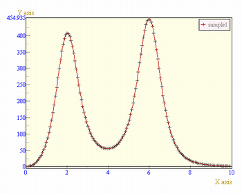
import ccs.math.*;
import ccs.math.impl.*;
import ccs.comp.ngraph.*;

public class HowtoFFT {

	public static void main(String [] args) {
		double R = 100;
		int num = 4096;
		// 準備
		AFunction af = AFunctionClass.getFunction("(sin(2*x)+sin(6*x))*exp(-x)");
		double [] ar = AArrayFunction.toArray(0,R,num,af);
		Complex [] cr = Complex.translate(ar);

		// フーリエ変換
		DFT engine = new DFT();
		Complex [] tr = engine.dft(cr);

		// パワースペクトルの表示
		double [] tar = Complex.translate(tr)[1];//虚部を配列に取り出す
		for (int i=0;i<num;i++) {
			tar[i] = tar[i]*tar[i];//2乗する
		}
		double dk = 2.*Math.PI/R;
		AArrayFunction afi = new AArrayFunction(0,dk,tar);

		//表示
		PlotContext context = Graph.show( af );//変換前の関数
		context.setAutoScale(0,false);
		context.setActiveRange( new RealRange(0,0.001,10,1) );
		context.updatePlotter();

		context = Graph.show( afi );//変換後の関数
		context.setAutoScale(0,false);
		context.setActiveRange( new RealRange(0,0.001,10,1) );
		context.updatePlotter();
	}
}
行列とベクトルのクラスを用いて、基本的な演算を行うことが出来ます。
import ccs.math.*;
import java.text.DecimalFormat;

public class HowtoMatrix {

	public static void main(String [] args) {
		vectorSample();
		System.out.println("===================================");
		matrixSample();
	}

	static void vectorSample() {
		//構築と値のセット
		MathVector a = new Vector2D(2,1);
		MathVector b = new Vector2D(3,4);
		//ベクトルの出力
		System.out.println("A: "+ a );
		System.out.println("B: "+ b );
		System.out.println();
		//足し算と引き算
		System.out.println("A+B: ");
		System.out.println( a.add( b ) );
		System.out.println("A-B: ");
		System.out.println( a.sub( b ) );
		System.out.println();
		//内積と外積
		System.out.println("AB: ");
		System.out.println( a.innerProduct( b ) );
		System.out.println("AxB: ");
		System.out.println( a.outerProduct( b ) );
		System.out.println();
		//長さ
		System.out.println("|A| = " + a.getLength() );
	}

	static void matrixSample() {
		//適当な行列の生成
		MatrixGD m1 = new MatrixGD(new double[][]{{1,2},{3,4}});
		MatrixGD m2 = new MatrixGD(new double[][]{{1,2},{2,4}});

		//適当なベクトルの生成
		VectorGD v1 = new VectorGD(new double[]{5,6});

		//表示
		System.out.println("m1: " );
		System.out.println(m1);
		System.out.println("\nm2: " );
		System.out.println(m2);
		System.out.println("\nv: " + v1);
		//足し算
		System.out.println("\nm1 + m2:");
		System.out.println(m1.add(m2));
		//行列の掛け算
		System.out.println("\nm1 * m2:");
		System.out.println(m1.mult(m2));
		//ベクトルとの掛け算
		System.out.println("\nm1 * v:");
		System.out.println(m1.mult(v1));
		//
		//フォーマットつき出力
		DecimalFormat df = new DecimalFormat("###.###");
		//逆行列(ガウスジョルダンの掃き出し法)
		System.out.println("\nm1;inverse:");
		System.out.println(m1.getInverse().toString(df));
		//逆行列をかけた結果
		System.out.println("\nm1;inv * m1:");
		System.out.println( m1.getInverse().mults(m1).toString(df));
	}
}
A: vec: 2.0 1.0
B: vec: 3.0 4.0

A+B:
vec: 5.0 5.0
A-B:
vec: -1.0 -3.0

AB:
10.0
AxB:
vec: 5.0

|A| = 2.23606797749979
===================================
m1:
matrix ----
 1.0 2.0
 3.0 4.0

m2:
matrix ----
 1.0 2.0
 2.0 4.0

v: vec: 5.0 6.0

m1 + m2:
matrix ----
 2.0 4.0
 5.0 8.0

m1 * m2:
matrix ----
 5.0 10.0
 11.0 22.0

m1 * v:
vec: 17.0 39.0

m1;inverse:
matrix ----
 -2 1
 1.5 -0.5

m1;inv * m1:
matrix ----
 1 0
 0 1
線型連立方程式を解くことが出来ます。「Ax=B」の形で係数Aと定数Bを、リスト2.2.5.2[連立方程式の例]のように計算クラスに与えるとXを解くことが出来ます。デフォルトの実装ではLU分解法を使います。
import ccs.math.*;
import ccs.math.linear.*;

public class HowtoSimEq {

	public static void main(String [] args) {
		double[][] am = {
			{1,2},
			{3,4}
		}; // 行列A
		Matrix a = new MatrixGD(am);

		double[] ab = {5,6}; // ベクトルB
		MathVector b = new VectorGD(ab);

		LinearEngine eng = LinearEngine.getDefaultEngine();
		MathVector result = eng.solves(a.getCopy(),b.getCopy());

		System.out.println("Matrix: A");
		System.out.println(a);
		System.out.println();
		System.out.println("Vector: B");
		System.out.println(b);
		System.out.println();
		System.out.println("Result: X");
		System.out.println(result);
		System.out.println();
		System.out.println("----\ncheck: A*X");
		System.out.println(a.mult(result));
	}
}
$ java HowtoSimEq
Matrix: A
matrix ----
 1.0 2.0
 3.0 4.0

 Vector: B
 vec: 5.0 6.0

 Result: X
 vec: -3.9999999999999987 4.499999999999999

 ----
 check: A*X
 vec: 5.0 6.0
1階、2階の常微分方程式を数値的に解きます。積分アルゴリズムを自由に選んだり、連立微分方程式を解いて、簡単な場の方程式を解くことも出来ます。(参照:###)
一階常微分方程式の場合、「dy/dx = f(x,y)」という式の形になりますが、簡単な例として「dy/dx = -y」の場合です。
import ccs.math.*;
import ccs.math.difeq.*;

public class HowtoDifEq1 {

	public static void main(String[] args) {
		//方程式の構築
		ScalarFunction eq = DifEquation.getEquation("-y");
		//初期条件(x=0, y=1)
		VariableSet init = new VariableSet(0,1);
		//数値解エンジンの構築
		//デフォルトのアルゴリズムはルンゲクッタ法
		DifEqSolver eng = new DifEqSolver();
		//解く (式、初期条件、xの終了範囲)
		AFunction af = eng.solve(eq,init,20);
		ccs.comp.ngraph.Graph.show(af);
	}
}
一階常微分方程式の場合、「d^2y/dx^2 = f(x,y,dy/dx)」という式の形になりますが、簡単な例として減衰振動の「d^2y/dx^2 = -0.4*dy/dx -y」の場合です。
import ccs.math.*;
import ccs.math.difeq.*;

public class HowtoDifEq2 {

	public static void main(String[] args) {
		//方程式の構築
		ScalarFunction eq = DifEquation2.getEquation("-0.4*dy-y");
		//初期条件(x=0, y=1, dy=0)
		VariableSet init = new VariableSet(0,1,0);
		//数値解エンジンの構築
		//デフォルトのアルゴリズムはルンゲクッタ法
		DifEqSolver2 eng = new DifEqSolver2();
		//解く (式、初期条件、xの終了範囲)
		AFunction[] af = eng.solve(eq,init,20);
		ccs.comp.ngraph.Graph.show(af[0]);
		ccs.comp.ngraph.Graph.show(af[1]);
	}
}